Author: maxoates1

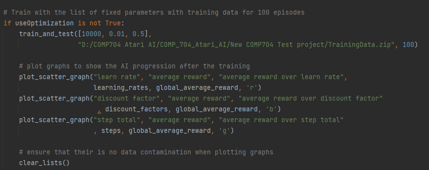
In this post I will be concluding my findings that I have obtained and what I have learned throughout the development of my AI.

DQN

Due to not having lots of experience or knowledge about Machine Learning AI techniques, Deep Q Network (DQN) was an interesting approach to creating an AI that could playtest a video game environment. This is because it incorporated both Neural Networks and Q-learning which would allow for less chance of short term oscillations occurring when monitoring a moving target (N. Yannakakis and Togelius 2018).

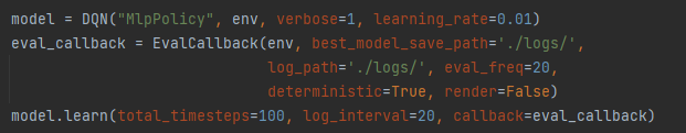
After using Stable Baselines3’s DQN class, I had found it very useful when trying to get it to work with OpenAI Gym’s Atari environments since it was designed to work with the type of AI environment library. In addition, it was quite easy to set up and get working, however the Atari environments must be the RAM versions to ensure they can work on standard computers. Adjusting the AI’s parameters was a simple process allowing for optimisation techniques to be easily implemented and used to ensure it could get good fix parameters. Additionally, the AI had parameters that I could adjust to manage when it should return evaluated results and when to stop training if it got a specific score.

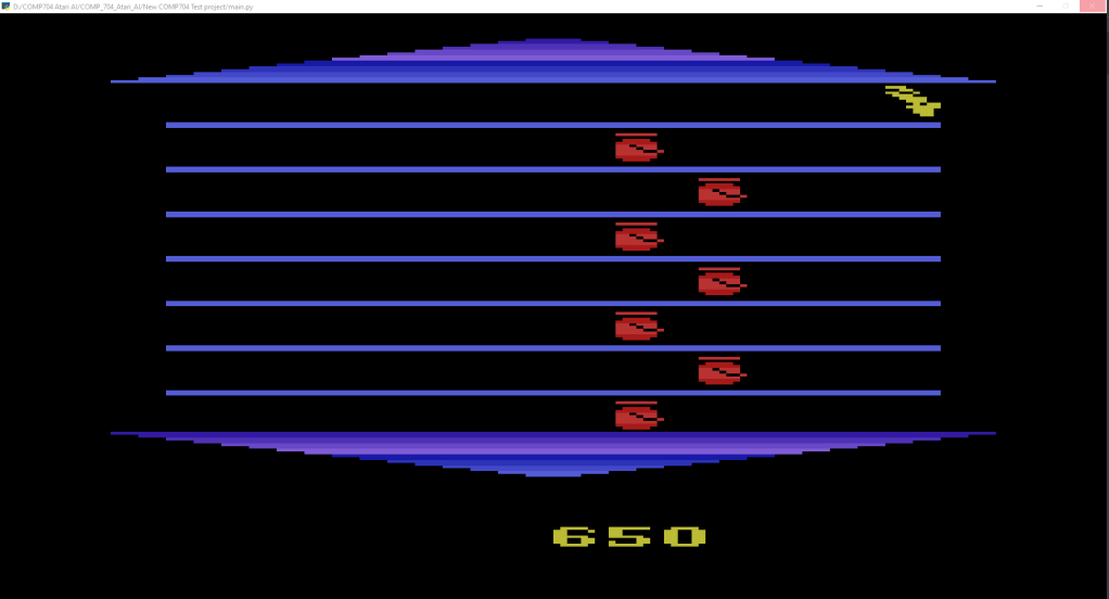
One of the limitations with the DQN I found is that it struggles to learn how to work with random events. I discovered this after researching how DQN performs when playing a card game compared to another AI technique called Proximal Policy Optimization (PPO) as that DQN AI struggled to play against an agent using random actions (Barros et al. 2021). I found this to be true, as when training my AI in the Asterix (1983) environment (a game that has random features) it was able to learn patterns about the game but was not able to handle all them and would occasionally make simple mistakes.

Another problem I experienced with the DQN AI was that it kept taking advantage of a design flaw in the game causing it to stay still in one of the top corners of the environment. This was so that it would be efficient while getting a big score.

Genetic Algorithm and Optimisation

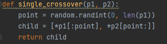
Using Genetic Algorithm (GA) as a parameter optimisation method has been a very useful technique as it has helped me pinpoint possible fixed parameters that I could use for the AI. This was achieved by using single crossover and mutation to generate new parameters based off the old ones and then test them to find the best one out of them all (Miller and Goldberg 1995). Additionally, by using this technique it saved me time from needing to adjust parameters by myself which would have been a much slower task.

Two problems I did have with using GAs was that it could take a while for the AI to create generations as well as train and test each one. However, this was likely due to the AI not having any training data or the reward threshold had not been set up to keep track of the most common reward being returned. The second problem I had faced, was the potential parameters could be quite limited and the results look quite similar to one another despite the mutations being applied. This may have been due to the range of mutations that could be applied or there not being enough example generations to use at the start of the system.

Looking into GA has introduced me to different techniques in AI as my knowledge base was quite limited. In addition, for future iterations of this AI and AI projects I will use it as a way to optimise finding the most useful fixed parameters.

Parameter adjustments

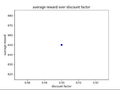
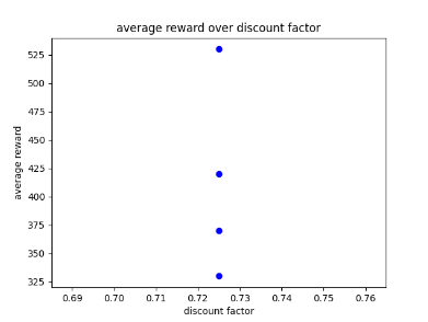
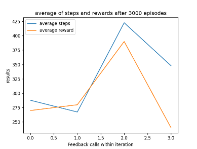
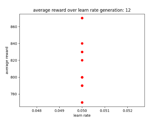
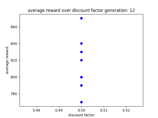
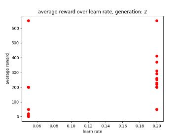
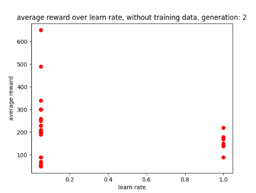
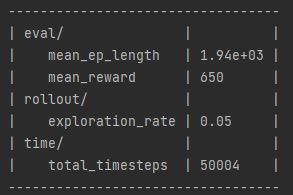
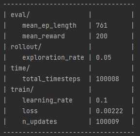
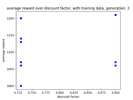
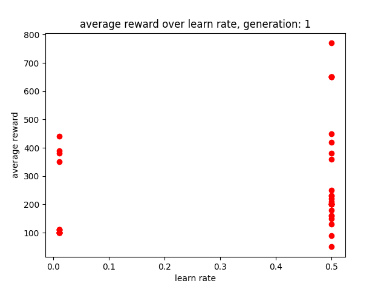
After using GA for 6 generations to find the best possible parameters I have learnt that the learn rate seems to work best between 0 and 0.5 and the discount factor works best between 0.5 and 1. After experimenting with fixed parameters with the constraints in mind, I found that the AI performs best when it has a step total of 10,000, a discount factor of 0.752 and a learn rate of 0.5. This is because it allowed the AI to achieve a score of 750 and learn patterns in the environment, however it was not able to maintain the score at a consistent rate. I chose 0.752 as the AI was achieving good scores that were between those numbers. Two examples of previous graphs are shown below. The AI was getting more consistent but low scores around a learn rate of 0.90, but having a learn rate of 0.75 resulted in the AI getting a higher score at a less consistent rate.

Step/reward monitoring techniques

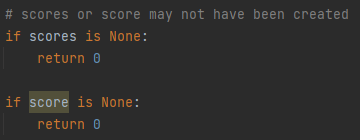
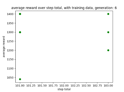
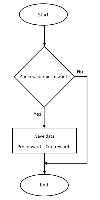
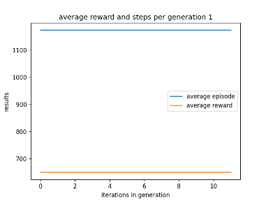
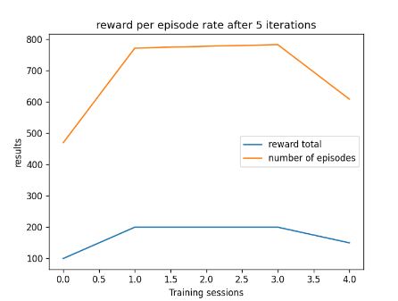
To improve how my AI saved its training data I introduced a custom feature intended to ensure that the AI does not override good training data with bad training data. This is because by observing my AI I noticed it slowly drops in progress near the end while still saving data. A graph of its progress drop is shown below in fig 3.

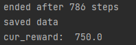
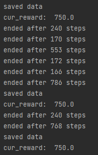
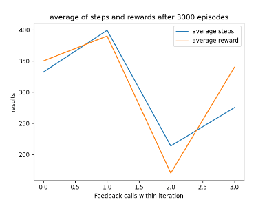
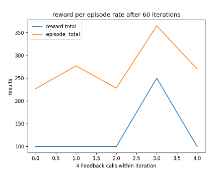
In addition, changing from monitoring steps to monitoring rewards has worked very well, allowing the AI to get a better score with a smaller number of steps. Using the reward technique has also prevented the AI from dropping in performance near the end of its training. An example can be found later in the post in fig 5.

Feature extraction

I decided to add a feature extraction technique as an extra layer of security to ensure the AI does not save training data if the AI has been standing still for too long. Looking at the results, the system did show some promise as the AI has performed better. However, it is a disappointment that OpenAI Gym’s environment reward function cannot be edited during training as I believe it would be more effective.

Feature extraction involves taking existing features in the AI and creating new ones in order to help the AI improve in its training (Ippolito 2019). While the system I had did not entirely do this due to scope and library limitations, it was monitoring how often the AI was standing still and preventing the AI from saving training data that stood still for too long. This was intended to encourage the AI to explore the environment more often.

Plotting graphs and CSV files

For my AI I had two different types of graphs to express the AI’s data and progress, line graphs and scatter graphs. In addition, the returned data was stored on csv files that could be used to plot the data on the graph.

Line graphs were useful to show off the progress of the AI over 4 evaluation callbacks but it does not work well when the data is not linear or with multiple parameters. I found it is very useful when showing the progress of an AI with fixed parameters.

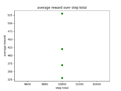
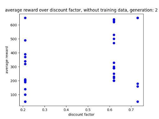
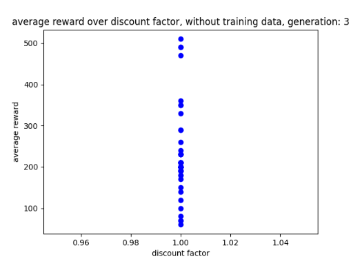
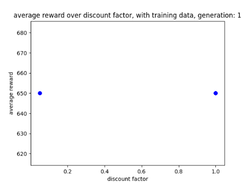
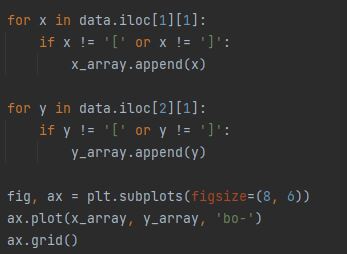
Scatter graphs were used for non linear data allowing for better representation of what parameters get what results. Though not entirely accurate, looking at the cluster of dots and looking at all the parameter graphs can give some guidance as to what parameters values work best. Below are two examples of the different scatter graphs.

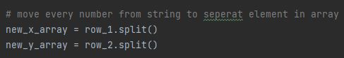
One problem that I did have with storing data on csv files, was that some data was stored on one cell of the csv file rather than each bit of data being stored on each cell in the table. Because of this I had to resort to building a filter that could break down the data and plot the data properly on a graph.

Further enquires

For future improvement, when it comes to parameter optimisation, I was thinking about having a system that would generate multiple AI and environments to see if this would allow for more effective training sessions and generate better parameters. Doing this multiple times with the same training data would enable me to see what results are returned. The one problem this could have would be computational requirements as having multiple AI running at the same time may put a strain on the computer’s RAM. (expand on multi agents running at the same time)

Upon further research AI techniques do exist to allow DQN AI to perform such tasks especially ones with randomness and low probability. For example, the system I found was experimented on to predict the stock market and was able to produce reasonable strategies for long term planning (Carta et al. 2021).

Reflection and Conclusion

Upon reflecting on my work, I have learned much throughout this development journey as I now understand how to build a DQN AI. In addition, it uses techniques like GA for improved parameter optimization as well as having systems to monitor and save data to ensure that the AI has the best training data.

While it is a shame that the AI cannot play Asterix (1983) properly or get a large score without overfitting, it is good to see that it can learn and play the game in general. In addition to that, the AI is able to improve itself using the training data and plot both line and scatter graphs to show the AI’s progress and which set of parameters provide the best results.

In conclusion, the AI is able to get a score between 200 to 750 while playing the game using the design flaw but also playing the game like a human would. In addition, the systems working alongside it have added it in collecting and plotting data for training purposes.

In future projects that require play testing I would be interested to see if I could incorporate my AI into them in order to try and get good feedback. However, this would require improvements and a library that would allow the AI to work with video game engines such as Unity or Unreal engine.

Bibliography

Asterix. 1983. Atari, inc, Atari, inc.

BARROS, Pablo, Ana TANEVSKA and Alessandra SCIUTTI. 2021. Learning from Learners: Adapting Reinforcement Learning Agents to be Competitive in a Card Game.

CARTA, Salvatore et al. 2021. ‘Multi-DQN: An ensemble of Deep Q-learning agents for stock market forecasting’. Expert Systems with Applications, 164, 113820.

IPPOLITO, Pier Paolo. 2019. ‘Feature Extraction Techniques’. Available at: https://towardsdatascience.com/feature-extraction-techniques-d619b56e31be. [Accessed Mar 4,].

MILLER, Brad L. and David E. GOLDBERG. 1995. ‘Genetic Algorithms, Tournament Selection, and the Effects of Noise’. Complex Syst., 9.

N. YANNAKAKIS, Georgios and Julians TOGELIUS. 2018. Artificial Intelligence and Games. Springer.

Figure List

Figure 1: Oates. Max. 2022. example of AI’s results between 0.6 and 0.9.

Figure 2: Oates. Max. 2022.example of AI’s results between 0.7 and 0.9.

Figure 3: Oates. Max. 2022. example of AI losing progression over time.

Figure 4: Oates. Max. 2022. example of scatter graph.

Figure 5: Oates. Max. 2022. example of line graph.

In this post I will be implementing a simple system that will monitor the AI’s actions and adjust the reward accordingly, this is similar to feature extraction. The main goal of this is to stop the AI from standing still for too long and remove points if it does so. This is intended to train the AI and stop it from using the design flaw and get stuck in a local maxima. I will then be looking over the graphs from this and previous results and fixing the parameters to those set values. Finally, I will add more polish to the AI by replacing its step measuring system with a reward measuring system instead to ensue that the AI saves the best of its training data.

Introduction

After talking to one of my lecturers, he suggested that I find a way to include a system that stops the AI from performing specific behviours by adjusting its reward. For example, the most consistent problem with the AI is that it will stand still for too long at the corners of the environment, resulting in taking advantage of the game’s design flaw, this is because it believes that is the more efficient strategy. Looking over performance techniques for DQN, I have decided to use a feature extraction like system to monitor every action the agent performs. For instance, if it is standing still for too many steps in the environment it will lose points. This is intended to encourage the AI to keep moving in hope of it playing the game more naturally and not using the design flaw.

Feature extraction and reward adjustment

As mentioned in the introduction I aim to create a system that is similar to feature extraction. Feature extraction works by reducing the number of features in a given AI system by taking existing ones and replacing them with new features (Ippolito 2019). While I won’t be adjusting or creating features, I will be monitoring current features and telling the AI to use or ignore current techniques to ensure that it will not get stuck in a local maxima.

The system worked as I could access the current action the AI was performing, however the reward system did not work. Further inspection of my research revealed that the DQN example my research was using, was a custom DQN class and not Stable Baselines3’s DQN class, meaning the reward for the AI’s current state and action could not be adjusted (Sachin 2019). Going with the alternative part of the plan I did get feature extraction to work with the fitness function in a different way. I included a disqualifier variable that would increase by one if the agent was standing still for more than a specified amount of steps. If the individual had a smaller disqualifier than the other one then it would be picked. Additionally, when saving data it would check if the disqualifier value is smaller than 1200, as testing has shown that it is usually the smallest number. Below are screenshots of the code when being applied as well a flowchart of how it works.

Results of training for 3 generation

After 3 generations the AI was able to move around the environment without using the design flaw and play like a normal player. However, it did walk into obstacles at times causing it to lose the game, while at other times it could avoid the obstacles very well. The AI making the mistake of hitting obstacles that should be easy to avoid might be the result of a small amount of available training data. However, this problem will likely be taken care of by training the AI further and seeing what happens. Below is the video and graphs of the results.

Fixing parameters and results of training for 100 episodes

Based on collected training data I will fix the parameters to the set values to ensure that their performance is consistent. While training the AI, I intend it to still use its step checker and feature extraction algorithms so that it will only save its best performances. I will then be training the AI for 100 episodes to see if this will improve its performance. Below in fig 7 is the fixed parameters being used for the AI.

I chose these parameters because from previous results the AI works best with a learning rate between 0 and 0.5 and with a discount factor that is between 0.5 and 1. Looking further into the previous results from parameter optimisation I have chosen a step total of 10,000, a learning rate of 0.01 and a discount factor of 0.5. This has led to good results and was the reason it got a score of over 1000 in the past. However, this was at the risk of the AI using of the design flaw.

After training the AI for 100 episodes, it seems that the AI switches between two behaviours similar to previous versions of the AI, these are: explore at cost of the score and be efficient and get a good score at the cost of exploration. For example, The AI will explore the environment and get a good score between 400 to 650. After playing the environment a few times (mainly five) the AI will switch and begin to be very efficient and use the design flaw in the game. Additionally, the AI seems to perform best when there is not a lot of obstacles in the way and will be able to avoid and collect points with a small margin of error. Below in fig 8 is an example of the AI switching between behaviours mid playthrough.

After observing the AI’s training session and how frequent it was saving the data, it made me curious if the AI would work better without the feature extraction. I was wondering about this as training the AI whilst still standing still for quite some time made me question the effectiveness of the system. After training the AI for 100 episodes without the feature extraction it turns out the AI had performed a slightly worse as it was getting a score between 200 and 400. A video of its performance is shown below in fig 11.

An observation I made during the AI’s training is that it can only reach 650 when training with just episodes and not with GA optimisation. This was making me wonder if having changing parameters allows for the AI to get better results as its parameters are always changing to make sure that it performs better then last time. This would make sense as having static parameters that do not adjust to a game with random encounters would not allow for the kind of adaption that GA could provide.

Training after 3000 episodes

To test the AI’s performance further I decided to adjust the AI’s fixed discount factor parameters and train it for 3000 episodes to see if the extra training would help it improve and explore the environment more often. The discount factor parameter is now 0.752 as it has worked well in the past as well when getting the AI to explore its environment more often.

After training it would appear that the AI was still getting scores between 400 to 600 and has now resorted to staying still at one of the corners of the environment and only moving when needing to avoid obstacles, which only worked sometimes. Looking at the AI’s performance I believe it has gotten stuck on a local maxima even with the help of the feature extraction system trying to prevent this. This could be due to the randomness of the environment making it hard for the AI to adjust completely and find an efficient path. Below are the graphs showing off the results as well as the video of its performance.

Polish

As mentioned in a previous post I wanted the AI to measure rewards instead of steps to know when to save training data. While the AI was working well with the step solution, I noticed that the AI was getting very high scores but was not saving the training data due to the step total not being big enough. To ensure that the AI saves the right data I replaced the AI step measure system with a reward measurer, for more effective training.

After training the AI for 3000 episodes, the AI would appear to have developed an interesting strategy where it will move around to collect as many points as possible and then stay still during its final life. This results in it getting a score between 200 and 750, which shows promise but is not consistent. In addition, the inconstancy is so common that the averaged graph of the collected training data does not show it achieving 750 as a score, this is shown below in fig 16.

As you can see from the graph, it varies in scores and as mentioned previously the graph shows that the AI can get a higher score with a smaller step total, hence why the system exists.

The problem with the inconsistent score may be due to the AI recognising patterns in the games randomness and using those patterns to handle the random feature of the environment. Below is a video of the AI’s performance as well as a picture showing the AI achieving a score of 750 during training.

While this may not be the best solution, since this AI is able to achieve a score of 750 (which is higher than previous scores) then this solution does show promise to allow the AI to improve further, especially with its current training data.

Adjusting parameters

I then adjusted the learn rate parameter to 0.35 and the discount factor parameter to 1 to see if a larger discount factor and smaller learn rate would have any improvement while still keeping it in the radius that usually gives the best results. However, after training the AI for another 3000 episodes, the AI still performed the same tactics as before and stayed at one of the corners of the environment to get the best results. Additionally, the score still wasn’t concise, causing the graph to show results between 200 and 400. However, it was getting a score of 750 at a more consistent rate at first, but the score decreased over time to a score between 200 to 400. Below shows the set parameters, the times it saved the data and the graph of the results.

Further enquires

Looking at the AI, it only solves one goal which is to get the highest score possible. However, I am curious if it would be possible to give my AI multiple objectives in order to increase the agent’s chances of staying alive longer and thus getting a better score. For example, the AI could be given an objective such as keep moving when it stays still and when its moving around its objective would be to get the highest score possible. This might be possible, however it might mean readjusting how the system keeps track of objectives and how the rewards will be assigned.

Upon further research it seems that it is possible for this type of AI to exist but works best with more simple environments such as a simple game called “deep sea treasure”. In addition, for the scalar part of the AI instead of it measuring a single value, the system would need to measure a vector where each element represents the objective and pick the one with the highest value. While talking about objectives, the system can handle multiple objectives but they may need to be simple to avoid confusion. As for AI policies, the AI can work with the MLP policy but not the CNN policy (Nguyen et al. 2018). Overall the system shows promise and that it is possible to incorporate the system into my AI.

Reflection and conclusion

Upon reflection of my work, by adding the feature extraction system and improving the reward measuring system, the AI seems to be improving in its performance when saving and loading training data. This performance is improved further by adding fixed parameters based on the collected training data throughout the past weeks.

From looking at the results I am quite happy to see it improving, although it can be annoying that the AI can still occasionally make basic mistakes when in the environment and will still use the design flaw. Taking this further, the AI is still making mistakes, causing it to get lower scores than previous iterations, by this I mean the previous AI’s lowest score was 400 while now it can get 200. That being said, looking at the agent’s movement, the AI can recognise patterns in the environment’s randomness, allowing it to avoid obstacles and get rewards, thus allowing it to get a score as high as 750. Taking the training further and possibly changing the parameters slightly could allow for better performance. That being said, for the time being, having the AI’s parameters fixed at 10,000 for the step total, 0.5 as the learning rate and 0.752 as the discount factor will do very well for the time being. Although the reward may not remain 750 consistently at the start, it is able to score 750 throughout the entire game at an inconsistent rate, rather than eventually dropping over time.

In conclusion, with the improvements to the system and parameters, the AI is performing better than it has in the past, even if it is at the cost of the AI occasionally getting a lower score than before.

For future actions, since this is the last week of me working and experimenting on my AI, I will not be doing any more work on it. Instead, my next post will be a conclusion on everything I have learned on this course, the outcome of the AI and what I might do in the future if I want to take this AI further.

Bibliography

IPPOLITO, Pier Paolo. 2019. ‘Feature Extraction Techniques’. Available at: https://towardsdatascience.com/feature-extraction-techniques-d619b56e31be. [Accessed Mar 4,].

NGUYEN, Thanh Thi et al. 2018. ‘A Multi-Objective Deep Reinforcement Learning Framework’.

Sachin. 2019. ‘Reward Engineering for Classic Control Problems on OpenAI Gym |DQN |RL’. Available at: https://towardsdatascience.com/open-ai-gym-classic-control-problems-rl-dqn-reward-functions-16a1bc2b007. [Accessed Mar 02,].

Figure list

Figure 1: Oates. Max. 2022. flowchart of the feature extraction.

Figure 2: Oates. Max. 2022. screenshot of how action is measured.

Figure 3: Oates. Max. 2022. screenshot of consequences if standing too long.

Figure 4: Oates. Max. 2022. AI after training with feature extraction.

Figure 5: Oates. Max. 2022. learn rate after 3 generation.

Figure 6: Oates. Max. 2022. discount factor after 3 generation.

Figure 7: Oates. Max. 2022. step total after 3 generation.

Figure 8: Oates. Max. 2022. AI training with fixed parameters and not optimization.

Figure 9: Oates. Max. 2022. example of AI switching behaviours after 100 episodes.

Figure 10: Oates. Max. 2022. AI constantly getting a score of 650.

Figure 11: Oates. Max. 2022. screenshot of AI performance without feature extraction.

Figure 12: Oates. Max. 2022. discount factor results after 3000 episodes.

Figure 13: Oates. Max. 2022. learn rate results after 3000 episodes.

Figure 14: Oates. Max. 2022. step total results after 3000 episodes.

Figure 15: Oates. Max. 2022. video of AI after 3000 episodes.

Figure 16: Oates. Max. 2022. graph of AI’s performance.

Figure 17: Oates. Max. 2022. AI with improved reward measuring system.

Figure 18: Oates. Max. 2022. AI achieving a score of 750.

Figure 19: Oates. Max. 2022. new parameter data.

Figure 20: Oates. Max. 2022. AI saving data.

Figure 21: Oates. Max. 2022. results from training with new parameters.

In this post I will be increasing the amount of elements in the example generation for the learning rate and discount factor based on previous research. In addition I will be experimenting with population and generation sizes, for this the AI will have 12 generations each with a population of 4. This is to find values with good results that I can use for fixed parameters. Finally, I will be polishing the code by adding comments and reducing code duplication where needed.

Parameter experimentation and training

As mentioned in earlier posts the a current problem with the AI is that it is using a design flaw in the game in order to get a high score. This is due to it finding the most efficient path too quickly and not taking risks. By adjusting the discount factor and learn rate parameters it seems to explore the environment more often and get a good score because of it. That being said it still happens too often, as well as that, when the AI reaches its last life it begins to drop in performance and does not do so well as when it had more lives.

My solution to this problem is to experiment with adding more values to the example generation for the discount factor and learn rate as this has had good results in the past when working with the Genetic Algorithm optimisation. As well as that, instead of training the AI for 3 generations I will instead run it for 12 to see if there are any improvements in its performance. The generation example can be seen below in fig 1.

After Training the AI for 12 generations it seems to have reduced in terms of high scores as its highest score was 880 instead of 1200 or 1400. In addition, based on its results it seems to do well with a learn rate of 0.05 which is expected due to previous results. As for the discount factor it prefers a value of 0.5 for its planning horizon, this is also expected due to previous results. All of this is show between figs 2 to 4.

Looking at the AI’s performance when playing Asterix (1983) it seems that it switches between two behaviors, these being: explore a lot of the environment at the cost of a high score or be efficient and get a high score at the cost of exploration. Below are two videos that show its different performances.

As mentioned in earlier posts it is expected that when the AI is more explorative of its environment, it would be at the cost of its score. However, it has done better than expected since this AI is capable of achieving a score of 800 or 850 while still exploring the environment. This is good because in previous versions the AI could only reach a score between 400 to 650. While the solution has shown some promise, I think a better solution is required if I want the AI to have a better and more natural performance.

An observation I made during the AI’s training is that it is a lot slower when training without existing training data to use. To give an example, I noticed that it takes 1 hour for 5 generations to pass without training data, while it took 20 minutes for the AI to complete 5 generations when training with existing training data. This may be due to the AI having an idea of what to do in its environment when using training data. As for the AI without training data, it is starting from scratch and trying to find the most efficient path. I felt this was something to keep in mind when planning how long it will take for the AI to train and what I can achieve in the time frame.

Polish

Another problem I have been facing is to do with the AI using training data it has just created, as at the moment the user needs to tell the AI when to start using the training data. As I have found that it is very ineffective during experimentation as the AI may be training for 12 generations and the AI should start using the training data after the first generation but in current circumstances I would need to stop the training, set a parameter to true and then begin the training session again. In addition, I have noticed that the state of my code is not looking very professional and is in need of improvements.

My solution is to remove the Boolean parameter from the train_and_test function that tells the AI when to use training data, and replace it with code that simply checks if a file exists. This should mean that when the training data is saved after the first generation it will start using the existing data. For the system to know if a path exists or not I will use the os.path library. The code is shown below in fig 7.

Alongside this, to improve the quality of my code I have added comments so that it is clear what parts of the code do what and why. As well as that I have updated the code by moving large chunks of code to a separate function such as the lines of code that clear the lists used to store data for the CSV and graphs. This is to remove untidy code and to ensure that the lists can be cleared without need of duplicating code.

Further enquires

Looking at my AI’s functionality and how Reinforcement Learning (RL) relies on a minimum number of states for good performance, I wonder if a RL AI can play a card game with good performance due to its high amount of states and actions while still being dynamic for complex decision making (Mousavi et al. 2017). Upon researching existing papers it seems that RL can be used to play a card game, however some features like a greedy policy were mandatory in order for the AI to keep up. DQN did work well against both random and human opponents, however it was out performed by Proximal Policy Optimization (PPO) another type of reinforcement learning technique. (Barros et al, 2021).

If I were to try and use DQN to play a card game I would need to keep in mind how the AI would interact with the environment and the agent in it. Additionally, as the research shows, another technique performs better than DQN both with a human player and an opponent AI that uses random actions.

Reflection and conclusion

Upon reflecting on my work I can see that adjusting the parameters further does show some promise in getting the AI to explore its environment more often. However, as expected the AI did get a smaller score than when it is overfitting, but even then it was able to get a higher score than previous versions that explored their environments more often. That being said I am glad that the AI is improving.

However, while it is a success, the AI seems to switch between two types of behaviors when testing it in the environment. These two behaviours are: it will explore its environment more often or be efficient and use the design flaw and overfit. That being said, even when it does overfit it does explore the environment now and then.

In addition, polishing the code has made it look more professional, although in the end there was not much of the code’s architecture that I could change without affecting functionality. However, it is nice to see the improvement in the quality.

For my next post, ideally I would like to edit the environment’s code so that if the agent is standing still, it will lose points. This would be to ensure that it stops using the design flaw, however the environment script cannot be edited. Due to this, I will look into feature extraction as a way for the AI’s fitness function to try and time how long the agent is standing still. For example, if the agent is standing still for or longer than 2 seconds, do not save the data and try and give the AI a low reward through OpenAI Gym’s API.

The expected results can be achieved by using OpenAI Gym’s en.action_space function, where it will be used to check which action is being used in the current step (Brockman et al. 2016). Attached to this will be a counter which increases by one every time the action is nothing (noop). Now there are some potential problems such as OpenAI Gym’s API not working with DQN since it uses the stable baselines3 library, but it would be worth the experiment to see if it will work. In addition, the environment is created with OpenAI Gym which contains the function that states what kind of reward is given to the agent so manipulating the AI’s reward might be possible.

Bibliography

Asterix. 1983. Atari, inc, Atari, inc.

BARROS, Pablo, Ana TANEVSKA and Alessandra SCIUTTI. 2021. Learning from Learners: Adapting Reinforcement Learning Agents to be Competitive in a Card Game.

BROCKMAN, Greg et al. 2016. ‘OpenAI Gym’. CoRR, abs/1606.01540.

MOUSAVI, Seyed Sajad, Michael SCHUKAT, Enda HOWLEY and Patrick MANNION. 2017. Applying Q (Λ)-Learning in Deep Reinforcement Learning to Play Atari Games.

Figure list

Figure 1: Oates. Max. 2022. example generations with more parameters.

Figure 2: Oates. Max. 2022. AI after 12 generations.

Figure 3: Oates. Max. 2022. AI after 12 generations and a learn rate of 0.05.

Figure 4: Oates. Max. 2022. AI after 12 generations and a learn rate of 0.5.

Figure 5: Oates. Max. 2022. AI playing game with 12 generations part 1.

Figure 6: Oates. Max. 2022. AI playing game with 12 generations part 2.

Figure 7: Oates. Max. 2022. snippet of path checker code.

In this post I will be experimenting with discount factor parameters between 0.5 and 1. As well as that I will be trying the AI in a different environment to see if it can run and train with little to no changes. Additionally, I will changing the learn rate and discount factor based on pervious experimentation to see if that improves its performance. By doing this I should be able to find good parameters for the AI to use and get it to play the game in a more natural manner.

Training

In this experiment I was changing the generation example’s discount factor so that it was between 0.5 to 1. This is to see if this would affect the AI’s planning horizon and thus hopefully move around the environment more often and prevent from overfitting.

During the training I remembered that chances of the discount factor parameter being mutated in the genome are up to random chance. This means generation examples might be the only ones used. In addition, random mutation affected the experiment due to it mutating the discount factor from a value between 0.5 – 1 to 0.2, below the intended parameter scale. An example of this happening is shown below in fig 2.

Looking at the graph the AI performed quite well with 0.2 as its parameter which is expected as a smaller discount factor parameter means a more efficient solution which usually results in a very big score. That being said, the second generation it got rewards between 450 and 600 while the first generation got a score of 1200 which was before the mutation occurred. This means by chance, the AI was able to get a score of 1200 once with a discount factor between 0.5 and 1.

Running in the environment

Looking at the AI interact with the environment with a higher discount factor shows promise as it moves around the environment and does not exploit the design flaw. However, this is at the cost of big scores as its biggest score was 450.

Further training with data set

In this experiment I began training the AI further with an existing data set from previous training. The AI was trained for another 3 generations (6 generations in total).

During the training with the data set it almost immediately began using the design flaw to get a score of 1200. Additionally, I have noticed that when it has one life left it performs less well compared to when it had three and two lives left.

Looking at the graph it appears that doing well with a discount factor of 0.2 in previous generations has not affected the AI when performing as its performance switches between 0.5 and 1. Because of this I think it might not be a problem if the mutation does affect the range of the generation examples.

Despite all that, when playing the game in human render mode (so that we can see play at normal speed) it appeared to be behaving the same way it did with only a data set of 3 generations.

Looking at its performance its making me wonder if the discount factor is having a big impact on its performance to such a point that having training where it uses the design flaw does not have much impact. This would make sense since the discount factor affects the AI’s planning horizon (III and Singh 2020).

Running AI with 9 generations of training data

After running the AI with 9 generations worth of data and a discount factor ranging between 0.7 and 0.9, the AI did still take advantage of the design flaw. However, there were some moments where it would move from the top of the level (the design flaw) and move around the environment. This Allowed it to get a score of 1250, 50 points higher than when it just used the design flaw.

Testing the AI in a different environment

Looking back at one of my previous further enquires, due to having some time I decided to test my AI in a different Atari environment and see if the AI can play a different game without needing any changes to the code. My choice of environment is the Atari game Assault (Brockman, 2020).

While the AI is playing Assault, with its current generation example parameters, like Asterix(1983) it is possibly that the AI is being too efficient and staying in one part of the environment. I believe this to be the case due to it staying still in one part of the environment. This is shown in the video below in fig 9.

During its training the AI did work and showed promise, however there were events where an error would occur causing the AI to stop training all together. This is shown below in fig 10.

This was happening due to the AI returning a value of type None thus preventing the SUM function to work. The possible cause for the AI returning 0 was because it was getting a score of 0 while training. Though it was annoying that it was not working, this experiment has shown that it is possible for the AI to return None. So I have added some code to check that score or the list of scores is None. A picture of the code is shown below in fig 11.

Adjusting learn rate and discount factor parameters

The final experiment that I’m doing in this post is change the learning rate and discount factor parameters based on previous training data to so if the AI can improve on performance without overfitting.

Looking at previous training data, the AI works best with learn rate parameters between 0 and 0.5 and discount parameters between 0.5 and 1. based on this the example generation will be given parameters based on this. The example parameters are shown below in fig 12.

While training the AI for 6 generation I noticed it was able to achieve a score of 1400, how this was at the expense of it overfitting. That being said in order for it to achieve this it had to moved around the environment as pervious training has shown that just staying at the top of the level results in a score of 1200. A screenshot of training is shown below in fig 13 and a graph showing its score in fig 14.

Once it had finished training the AI was able to get a score of 1400 when playing Asterix(1983) at normal speed, this is shown in the graph below in fig 15. However, it did overfit for most of the run through, that being said, it did on occasions move around the environment to get points, which was expected as mentioned earlier. Below in fig 16 is a video of its performance.

Further enquires

While training the AI I had noticed that stopping the training, adjusting the parameters and the training again was a bit tedious. As a fix for this I was wondering it would be possibly to have the example generation parameters change based on the smallest and biggest values the user gets. This idea could be useful if the user wants to change the parameters when trying to narrow in on a good set of example parameters, however it could be vexing when trying experimenting with random ranges in parameter sizes and the system begins to close in on a potential fix when that was not the intention.

Reflection and conclusion

Reflecting on my work I can see that by adjusting the parameters for the learn rate and discount total has improved the AI performance. However despite the changes to ensure it stops using the discount factor, it seams that the AI will still overfit and use the design flaw in the game.

In addition, I wanted to se if the AI would be able to play a different game and though it was not successful it has revealed that its possible for the AI to return a type of None when returning its fitness. Because of this measures have been put in place to ensure that None is not returned.

Despite these problems and feeling vexed about them, the AI has been able to improve, now being able to gain a score of 1400 by using the design flaw and moving around the environment optionally. Additionally, due to the randomness of the game it would be hard to predict what move to make next, which might be empowering its decision to stay still at the top of the level.

In conclusion, the AI has improved by adjusting its parameters, however has mentioned in the previous post, it might be very difficult for the AI to get a large score without using the exploit. Because of this it may be best to look at other alternatives.

For my next action I will continue to experiment with the learn rate and discount factor parameters, such as increase the number of elements in the generation example that the AI uses when creating a generation. In addition, I will begin commenting and polishing the code to make sure it looks more professional.

Bibliography

Asterix. 1983. Atari, inc, Atari, inc.

Brockman, G. et al., 2016. Openai gym. arXiv preprint arXiv:1606.01540.

III, Hal Daumé and Aarti SINGH. (eds.) 2020. Discount Factor as a Regularizer in Reinforcement Learning. PMLR.

Figure list

Figure 1: Oates. 2022. generation example for discount factor parameter.

Figure 2: Oates. 2022. mutation causing smaller discount factor.

Figure 3: Oates. 2022. generation 1.

Figure 4: Oates. 2022. generation 2.

Figure 5: Oates. 2022. generation 3.

Figure 6: Oates. 2022. AI playing game with low score.

Figure 7: Oates. 2022. example of AI switching between 0.7 and 0.9 discount factor.

Figure 8: Oates. 2022. AI taking advantage of design flaw.

Figure 9: Oates. 2022. AI training to play Assault.

Figure 10: Oates. 2022. example of None error.

Figure 11: Oates. 2022. picture of code used to check None is not being returned.

Figure 12: Oates. 2022. altered example generation parameters.

Figure 13: Oates. 2022. AI achieving a score of 1400.

Figure 14: Oates. 2022. graphs showing score of 1400.

Figure 15: Oates. 2022. AI after 6 generations.

Figure 16: Oates. 2022. video of AI getting a score of 1400.

In this post I will be training my AI further to see if it can be improved by exploring the environment more often and solve the problem with the AI using the environment’s design flaw too often. This will be done by experimenting with the AI’s learn rate, step total and discount factor parameters.

Speeding up training and design flaws

While the AI is training, it can take up to an hour for it to complete the training process which can be a problem at times due me not having a lot of time to train the AI. This is due to training and testing every individual in the population, which is done every generation. This means that 15 iterations are done each training session and what may vary the training time is each individual having a different step total value between 100 to 100,000 which makes the training session even longer.

So to try and speed along the training process I used stable baseline3’s ‘StopTrainingOnRewardThreshold’ function which keeps track of the AI training and if it receives an award of set amount it will stop the current training and move onto the next training session (Hill et al. 2021). During training I noticed that after 2 generations it gets really good at getting a score of 650 during its training. Noticing this I set the threshold at 650, which resulted in the training session taking between 10 minutes to 30 minutes depending on the AI’s progress, thus speeding up the process entirely. A picture of the code is shown below in fig 1.

Additionally, this solution works really well because, as the high-score changes I can simply change the reward_threshold parameter to fit, making this solution very adaptable.

As mentioned in the past this AI can overfit, but as I was observing the AI’s training I noticed that one thing that might be causing it to overfit was not so much due to lack of data or performance, but more to do with a design flaw in the environment. Looking at the video below in fig 2 you can see that the game’s obstacles spawn less at the top row of the environment, compared to the other rows. In addition, there are cases were the item that gives the AI’s reward spawn more frequently at the top row as well. I believe that the AI has found this design flaw and used it to get a high reward by standing still at the top and waiting for the points to come to the agent, as that would be more efficient then moving around the environment.

During the training the AI recorded and displayed the training data on scatter graphs per generation. The first 3 pictures below show its training and saving the data without any existing data sets to use.

However, when the AI begins using the training data by the end of the first generation it is able to maintain a score of 1200. This was achieved by the AI taking advantage of the design flaw (which is shown in the video previously mentioned) so that it could get a big reward.

Additionally, it shows the that a low learning rate may allow for better performance as there are more dots to the left (lower learn rate) than there are to the right (high learn rate). Giving the AI’s learn rate parameter smaller values may allow it to train faster, especially with a smaller data set. Though this may not stop it from using the design flaw, I will keep it in mind when setting up the AI’s parameters to ensure that it can train faster.

Adding more varying values to the example generation

In this experiment to try and stop the AI from using the design flaw, I added more values to the learning rate and discount factor example generation, this was to see if there were any improvements in its exploration abilities while still maintaining a good score.

During the training, the AI seemed to work best with a learning rate of 0.05 as shown in the 2nd and 3rd generation graphs, these are shown below in fig 8 and 9.

Additionally, the AI seems to have comes to a discount factor of 1 which is shown below in fig 10.

With the AI having a discount factor of 1 in its training data, it seems to explore the environment a lot more during the first game before using the flaw again in the second game. However, this seems to be at the expense of it achieving a high-score as this version only gains a score between 450 and 650 at best after 3 generations. This is compared to the previous version which got a score of 1200 after 3 generations but explored the environment less. A picture of the graph is shown below in fig 11 and its progress is shown in a video in fig 12.

Less discount parameters

Upon researching discount factors, one of the research papers suggested that having a smaller value would allow for better performance when exploring the environment (III and Singh 2020). When hearing about this I decided to give my discount factor examples smaller numbers (between 0 and 0.5) and a less amount of numbers in the example generation to see if this solution allows the AI to improve its performance after training. A picture of the AI’s smaller discount factor is shown below in fig 13.

Ideally if the AI could explore the environment more often and use the design flaw less often then the AI would be a success as it would play the game properly. Looking at how the AI plays the game, at this rate getting the AI to achieve a score of 1200 without using the flaw may be asking too much and instead achieving a score of 650 while playing the game properly would be a more achievable goal.

After training the AI for 3 generations the AI switches between 0.01 and 0.05 in order to achieve a score of 650. this is shown below in fig 14.

After using the training data on the AI, it would appear that having a smaller discount factor would cause it to use more efficient methods of playing the game, thus it used the flaw almost immediately. This can be seen in the video below in fig 15.

Graphs with different parameters and storage

As partly seen in the graphs above, I have now got the step total and discount factors plotted on scatter graphs and compared to the rewards. Alongside this I gave the graphs different colours: red for learning rate, blue for discount factor and green for step total, this improvement is to ensure the AI’s progress is more readable each generation.

While I was working on this, errors were coming up stating the sizes were different, however it turned out I simply forgot to clear the lists that where storing the data, causing new data to be added to the old data. With this solution the graphs worked perfectly though in order to make the solution more professional I might move the code to a function so that it looks neater.

Alongside this I stored the parameter data onto a csv file to ensure that the data could be viewed after training and plotted on a graph. A screenshot of the csv file is shown below in fig 16.

Further enquires

Looking at how the Genetic Algorithm (GA) optimization is used I wonder if it would be possible to add a database to the optimization and then use it to generate an average genome based on the performance of the individual. This could be a legacy system that keeps track of the best performing individuals 5 generations back and compares it to the current generation. This would be to see if anything from the previous generation could be used on the present to improve them, incase the AI starts dropping too much in performance. Of course this might cause problems with the mutation aspect of the GA, as it is meant to look for unique individual traits that could allow for better performance (GAD, 2018). However, I was curious if there was a way for unique traits to be applied to the next generation while ensuring the best traits of all the generations remain.

Reflection and conclusion

Reflecting on my work by experimenting with more values for the parameters allows for varying performance and scores. In addition, trying smaller values for the discount factor results in the AI being too efficient and picking a solution too quickly.

Looking at how the AI plays the game when not using overly efficient methods it may be difficult for the AI to get a score of 1200, so instead simply aiming for 650 could be a more achievable goal. Though it would be great if the AI could achieve big scores when playing the game properly, it feels inevitable that it would always use the design flaw to achieve its goal of high rewards.

Additionally, plotting more graphs to show how all the parameters are affecting the reward value and giving them different colours makes it much easier to follow the AI’s progress and tell which graph is which.

Looking at the AI’s performance it seems to either be doing well at the cost of overfitting and using illegal moves or playing the game more properly but at the cost of smaller scores.

Going further into my experimentation I would like to try giving the discount factor parameter, values that are between 0.5 and 1 to see if it will stop picking the most efficient method too soon. In addition, I might update the reward threshold to 1200 to ensure that the AI can train much faster, however this depends on the most frequent returned reward value.

Bibliography

III, Hal Daumé and Aarti SINGH. (eds.) 2020. Discount Factor as a Regularizer in Reinforcement Learning. PMLR.

GAD, Ahmed. 2018. ‘Introduction to Optimization with Genetic Algorithm’. Available at: https://towardsdatascience.com/introduction-to-optimization-with-genetic-algorithm-2f5001d9964b. [Accessed Feb 11,].

HILL, Ashley, et al. 2021. ‘Stable Baselines’. Available at: https://github.com/hill-a/stable-baselines. [Accessed 22/02/22].

Figure List

Figure 1: Max Oates. 2022. screenshot of reward threshold.

Figure 2: Max Oates. 2022. video of my AI exploiting a design flaw.

Figure 3: Max Oates. 2022. generation 1 of AI without training data.

Figure 4: Max Oates. 2022. generation 2 of AI without training data.

Figure 5: Max Oates. 2022. generation 3 of AI without training data.

Figure 6: Max Oates. 2022. graph of AI achieving a score of 1200.

Figure 7: Max Oates. 2022. picture of example generation.

Figure 8: Max Oates. 2022. generation 2 of training data.

Figure 9: Max Oates. 2022. generation 3 of training data.

Figure 10: Max Oates. 2022. discount factor after 3 generations.

Figure 11: Max Oates. 2022.example of discount factor graph using training data

Figure 12: Max Oates. 2022. example of AI getting a score of 450 while exploring.

Figure 13: Max Oates. 2022. picture of generation with a smaller discount factor.

Figure 14: Max Oates. 2022. graph of AI switch between different discount factors.

Figure 15: Max Oates. 2022. example of AI being efficient with a smaller discount rate.

Figure 16: Max Oates. 2022. example of parameter dat being used on the AI.

In this post, I continue to train my AI while making improvements to the mutations aspect of the AI so that it will function better. During this I will make improvements to the graph to ensure the data is more readable.

Training improvements

After having a talk with my lecturer I realized instead of mutating the entire population I should just mutate a random part of one individual, thus giving more of a nudge rather than a push. Upon further inspection of my research that was definitely the case as the diagram in the previous post shows it just affecting one part of the individual’s genome and not the entirety. This is to ensure that offspring has its own unique traits while also retaining some traits of its parents to ensure the benefits of the parents’ genome is passed on to the offspring (Bryan 2021). A picture of the code can be seen below in fig 1.

This did partially stop the AI from overfitting, however it did still stay in a corner as it found that tactic was the most efficient strategy. This is due to it not losing any points from standing still for too long. Besides that the AI did occasionally move throughout the environment trying to gain a high score like a player would.

In its current state it can only seem to gain a score of 200 while moving through the environment but I have increased its mutation random number generator from -10 to 10 to -100 to 100. This was to see if it would allow for a great amount of performance and differentiation, but this did not prove to be the case and so the mutation random number was set back to -10 to 10 and was gaining a score between 200 and 650. In figs 3 and 4 the graphs below show this process, please note that during this point the title was pending on improvements.

I implemented a save and load feature that allowed the AI to save its training data and when the user felt the time was right, could enable the load feature so that the AI could train and improve itself further.

However there was a problem, for a time, the AI only seemed to score 200 points while still overfitting. This was because, I had noticed that the training data was causing the AI to give worse results than when it trained from scratch.

At first I tried to reposition the save and load code to see if the functions were being called before the training had started, thus affecting how the training data was being used and updated.

However, looking back at the plotted training data, I realized that the AI had a tendency to peak and then drop in performance at the end. This made me wonder if the reason the training data was giving off bad results was because it was saving the end bits of the data and thus overwriting previous and better training data. The progression and drop can be seen in fig 3. To solve this issue I tried to see if there was a way for it to ignore the drop and only save the training data during the progression stage.

My solution was to have the AI compare its current reward to its previous reward and if the current reward was greater then its previous reward it would save the data. Below in fig 4 is a flowchart diagram of how the algorithm will work.

While it seemed simple at first, there was a problem, the variable containing the previous reward was being set back to 0 when the training function was being called. It did not matter whether it was global or local, the same results were happening. By having the previous reward variable set to global it would prevent Python from thinking the previous reward variable did not exist and needed to create a local variable in the function (Lutz 2014).

After some debugging it was clear that the global variable was working and it was being set to 0 by the current reward variable as that variable was switching between 0 and 50 during training and did not mimic the score in the game. This meant that I need to find a different way to get the agent’s reward. My temporary solution was to have the algorithm compare the number of steps the agent had preformed when training and see if the agent’s current steps were higher than the previous one. I used this method because usually if the number of steps are high, then so is the AI’s score, which is shown below in figs 5 and 6.

Additionally, getting the step total was much easier than getting the reward. After getting it set up, the save data algorithm could be more dynamic and work with other training sessions. This is shown below in fig 7.

I do want to try and see if I can get the algorithm to compare rewards as I’ve noticed cases where the AI can achieve a high reward with a small amount of steps. I could try evaluation_policy which is a function that can return reward values, however looking at its parameters, I’m unsure if it will create a separate environment or connect with the current one.

Nevertheless, saving the training data when it has a large number of steps seemed to have worked as by 3 generations and 5 iterations per generations, the AI was drifting between a score of 200 – 650. Continuing the training and loading the previous training data, by 6 generations the AI was constantly getting a score of 650 showing that it was progressing over time.

The last improvement I did for the training section was to add a discount factor to the AI’s parameters and GA optimization. This was to ensure that the AI would take risks and optimize its performance, as in its current form it was moving to one corner finding and concluding that this was the best solution too quickly. A discount factor is used in reinforcement learning to help reduce the number of steps required when training (François-Lavet et al. 2015). In addition, a discount factor can also be used to help optimize the performance of the AI, especially when using small amounts of data as it is the value that affects the AI planning horizon (III and Singh 2020). While this did show some improvement it did still overfit at times.

Graphs improvements

I began improvements on the graph so that it would only show the average step total and reward after every iteration. This was quite an easy process as I only needed to remove the code that called the plot function when an iteration was complete. Visualizing the progression data was much easier, as you now had only 3 to 4 graphs per iteration that showed the AI continuing in the new iteration from were it left off in the old one and either progressing or regressing. Additionally, I improved the title and labels so that their names were more descriptive of the data being shown.

I then began to see if I could get the graph to show the average episode total and reward every generation so that the user only has to look at 3 graphs. Additionally, I adjusted the labels so that you could tell how many iterations had passed in the generation and which generation the graph was representing. Below in fig 8 is an example of the AI’s performance when using existing training data.

While talking about representation, to ensure that the data was readable, I set up a scatter graph to show the rewards that were being generated compared to their learn rate. In an early version the data was collected per iteration and while it did work, there was problem. For some reason, while the data was plotted, the title or labels did not appear, this is shown below in fig 9.

This is possibly due to something in the code affecting how the labels are displayed, instead of it being a size error on the x and y axis. The reason I believe this is the case, is because if the x and y axis did have different shapes then the graph wouldn’t have been built at all and an error would have appeared.

After looking at other examples of scatter graphs I found a solution by using MatplotLib’s subplots function. While subplots, as the name suggests, is meant for multiple graphs instead of one, it has proven to be a good solution and could be used properly in the future if I want to display multiple different datasets on one graph (Yim et al. 2018).

In fig 10 you can see a graph of the working scatter graphs and in fig 11 you can see the code used to make the graph.

As you can see in fig 10, the AI was making some progress with a learning rate of 0.01, however it got better results by using a learning rate of 0.5. This is visualised by the cluster of dots around a reward between 100 to 200 and a reward of 400.

Further enquires

All the systems have been set up properly to train, store and plot the AI’s data now and so I could begin working on seeing if the AI could be used in other Atari environments. In theory the AI would not need any changes due to the architecture of Stable Baseline3’s DQN AI as when setting it up to play Asterix (1983), it was able to run the environment and set up the states and actions with ease. My only concern would be how the graphs will plot the data as there could be a chance that the data would be stored differently, however this can only be found out with experimentations.

Reflection and conclusion

Upon reflecting on my work I am quite impressed with the AI performance as, though it may still be overfitting at times, its ability to get high scores almost constantly over time is very fortunate. However, as stated earlier, it does overfit at times, which I intend to try and fix or at least improve on by adjusting its discount factor parameter to ensure that it doesn’t pick an efficient path too soon. This would be done by first adding more examples to the example generator so that it has a larger array to choose from at the start of training.

As for graphs, having a scatter graph that shows how well the different learning rates are affecting the reward has been very helpful as it allows me to tell which learning rate works best. That being said, there are limitations, as at times it does show only two learning rates affecting the reward, however this may be due to the generations picking the best learning rate based on fitness. In addition, current graphs are the result of the AI using existing training.

If I have the time I would like to plot the step total and discount factor to the rewards as well to see how they affect the rewards as well.

In conclusion I will aim to improve the AI’s dismount timer to ensure that it is more explorative and does not overfit too soon. Alongside that I will aim to have the AI’s training from beginning to end put on a graph to see what the results will look like.

Bibliography

Asterix. 1983. Atari, inc, Atari, inc.

BRYAN, Graham. 2021. ‘Randomized Optimization in Machine Learning’. Available at: https://medium.com/geekculture/randomized-optimization-in-machine-learning-928b22cf87fe. [Accessed Feb 11,].

FRANÇOIS-LAVET, Vincent, Raphael FONTENEAU and Damien ERNST. 2015. ‘How to Discount Deep Reinforcement Learning: Towards New Dynamic Strategies’.

III, Hal Daumé and Aarti SINGH. (eds.) 2020. Discount Factor as a Regularizer in Reinforcement Learning. PMLR.

LUTZ, Mark. 2014. Python Pocket Reference . (5th edn). United States of America: O’REILLY.

YIM, Aldrin, Claire CHUNG and Allen YU. 2018. Matplotlib for Python Developers: Effective Techniques for Data Visualization with Python, 2nd Edition. Birmingham, UNITED KINGDOM: Packt Publishing, Limited.

Figure List

Figure 2: Max Oates. 2022. improved mutation code.

Figure 2: Max Oates. 2022. example of AI ranging from 650 to 200 points.

Figure 3: Max Oates. 2022. example of AI varying progressing.

Figure 4: Max Oates. 2022. Flowchart of save data algorithm.

Figure 5: Max Oates. 2022. example of greater step length with high reward.

Figure 6: Max Oates. 2022. example of smaller step length with small reward.

Figure 7: Max Oates. 2022. example of AI saving data when steps are higher.

Figure 8: Max Oates. 2022. example of graph of generation 1.

Figure 9: Max Oates. 2022. example of labels not appearing on scatter graph.

Figure 10: Max Oates. 2022. example of working scatter graph.

Figure 11: Max Oates. 2022. code used to plot scatter graph.

On this post I added improvements to the filter and begin training the agent. In addition, I will be talking about using Genetic Algorithm (GA) as a method of optimization for the AI’s parameters while training

Filter problems and improvements

I began adding improvements to the filter by adjusting the variable names so that they were more accurate to their use. Additionally, I’ve replaced re.sub with string.replace due to it causing errors when switching from my personal computer to a university computer, this is likely due to my computer having a different version of Python compared to the university computer. A screenshot of the improved code this is shown in fig 1.

In addition, the filter is now able to plot graphs of all the data over each eval callback and plot a graph that shows the average episode and reward over each callback. Two examples of the graphs are shown below in fig 2 and 3.

When working on the filter and how it would work with the graph I was not sure if I should have the graph function preform a loop (based on current amount of data) when plotting each graph or if the filter should just call the plotting function to avoid code duplication. In the end I had the filter call the plot function when it had finished filtering the data but was still in the loop. This way each graph was plotted one at a time.

While I would have liked the function return a value for the plot graph to use, for the time being it is a good solution I intend to add improvements as develop goes on.

Plot function problems and improvements

For the plot function I had to rethink how the plotting function would use its parameters to work with the filter function as the filter was now calling the function. This problem did not have much of an impact on the scope of the AI development as I believed that I was able to rearrange the system architecture quite quickly.

To ensure that the plot function was compatible with the filter I removed the data parameter that contained the csv data and replaced it with two parameters for the y-axis data (where the filtered data is used) as well as three other string parameters for the labels and the graph’s title. This was to ensure that the graph could be as dynamic as possible while not going too far causing the function to be overly complex.

The quality of the solution had worked quite well and will remain as the current solution for the AI and how it plots graphs. This is to ensure that the user could have more control over how the graph was plotted.

Training and genetic algorithm optimization

Now that data can be displayed and the AI is functional, I began training my agent to play Asterix (1983) and adjust its step amount & learning rate parameters to determine how often it should train to get the best results. However, although it might be simple to change some of the parameters randomly to triangulate on the best parameter value by hand, due to the complexity of the game this would be a problem, as it would take quite a bit of time to find the best parameters.

Fortunately there is an alternative, which is using algorithms to optimize the best parameter values. I had two choices, the first was to use hill climbing, which will pick random values to use as the parameter and try and find the best value by climbing up from that value, however there are chances it will get stuck. To prevent it from getting stuck in a local optimization that only fits the current machine learning agent, you can set how many times it can guess a starting point. While this algorithm does work, as mentioned earlier it can get stuck and it’s starting points are random preventing you from having some control of its output (Bryan 2021).

The second option is Genetic Algorithm (GA) which is based off biology and takes a population approach, by combing individuals in a population with each other through crossover & mutated to generate some new and hopefully better parameters (Bryan 2021).

An example of crossover and mutation is shown below in fig 4.

In this case there were two populations one was the learning rate and the other was the step rate.

The tournament is used to find the best individual within the populations based on its performance in hopes that the next generation will adopt their best traits. This is achieved by testing the individual and seeing what results come back. After this, the individual will be added to the mating pool for crossover and mutation (Miller and Goldberg 1995).

The crossover is achieved by dividing both the parent’s genomes into two and then swapping the chosen halves with one another (Gad 2018). Since this genome contains both the learning rate and episode rate, the division will be done based on this rather than dividing the genome at random.

Crossover is done to ensure that the offspring is different from the parent populations and doesn’t share any identical traits. After that mutation is applied to the offspring to by selecting one of the genes and changing its value at random. This is a second layer of variation, because without it the offspring would just contain traits of both parents. This would mean no individual traits that could be helpful when being used for the new parameter or as a parent to make the next offspring more diverse (Gad 2018).

To show of how the optimization works with the AI system, below in fig 5 is a UML of the system architecture.

Example of training

I began training my AI using the GA optimization and it has successfully be able to train the AI to play Asterix(1983). Though the training did take some time especially with new generations being created, in about 2 minutes it was able to reach the highest score in the game (650 points). A screenshot is shown below in fig 6.

However, the AI maybe playing too well, over time it found a limitation in the game where staying in one of the corners and wait for the collectables to move to the agent was better than moving around. Because of this is means the AI is ‘overfitted’ and may need to have its parameters adjusted so that it preforms less efficiently (Gerrish 2018). A video of it overfitting is shown below in fig 7.

Problems with GA optimization

The crossover function was returning individuals that were either empty or combined the wrong way e.g. [learn rate, episode rate] []. In order for it to work, the episode rate needed to be the first element in the array and the learn rate the second one. by using * operator both arrays could be combines properly without any problems. In addition the : operator was used in the lists to get every element up until a random point in both populations. This was done to ensure variations could be applied to the individuals that where being added to the next population, this made the scope of the problem quite small as an effective solution was found relatively soon. An example of the code could be shown below in fig 8.

Another part of the optimization that I was having trouble with was the mutation part of the algorithm. I was trying to increase or decrease the step total and the learning rate to add individual traits to the offspring, however I seemed to be facing a problem, as for some reason the mutated learning rate came back as negative, which causes the AI to break down and stop. This is shown below in fig 9 and fig 10.

I believe this was happening because of the while loop parameters and that possible the ‘randomlearnrate’ variable due to the variable being initialized before the while loop and thus it possibly wasn’t being considered.

To see if this was the case, I replaced the while loop parameters with an if statement inside of the loop to ensure that ‘randomlearnrate’ wasn’t being initialized before hand.

This change worked as negative numbers were not being produced and the mutations where successfully added to the DQN parameters making the solution an effective one that will stay as is for the foreseeable future. This is shown below in fig 12. For reference, the ‘mutation’ print shows that the mutations are being applied.

As for the step total, there was no problem with mutating that value as it didn’t need to be within 0 to 1, meaning simply adding a random number to it was not a problem.

Improvements

An improvements I did to the code was change the number of total steps, as on further inspection of the parameter I realized that the parameter must be an integer (whole number) and while I have experienced no errors I want to make sure that everything was ok and that the data was accurate.

Further enquires

Looking at how GAs work and how an their performance I was curious if there could be other methods (besides hill climbing) that could allow for better AI optimization. Ideally I would compare different optimization techniques to see if faster ones could be used and if they yield better quality from their faster results. Of course a limitation would be time constraints since each one would require being implanted and set up to the AI. Addition, each one may require a different AI technique. An example of another algorithm for optimization would be MIMIC which works by remembering previous searching in order to optimize and break down the complexity space within the function rather than looking at a single input (BRYAN, 2021).

The point of the experiment is to see if a different optimization technique can just as good or better results at a faster pace.

Reflection and conclusion

Upon reflection of my work I’m happy the filter is working and that the plot is able to successfully plot graphs based on the data from the csv file. In addition, I found it very interesting to incorporate the GA algorithm on to my AI so that it step total and learning rate parameters could be optimized automatically, especially since this is my first time using it.

Though the AI is able to play Asterix(1983) very efficiently, I should begin experimenting to see if I can reduce the efficiency of AI so that it is not overfitting while still being able to play the game well.

In addition, the filter and graph work really well, however I learned quickly that I may need to adjust how often a graph is plotted since within one generation, 580 graphs had been plotted, a picture is shown below.

To improve on this I will adjust the graph and how the filter uses the function so that it plots a graph of the average of the AI’s performance after every iteration or after every generation.

For my next bit of work I will be adding improvements to the filter and how the graph uses it so that the user is not over whelmed with graphs. Additionally, I will be adjusting the optimization of the AI so that it can play the game with reasonable results while not overfitting.

Bibliography

Asterix. 1983. Atari, inc, Atari, inc.

BRYAN, Graham. 2021. ‘Randomized Optimization in Machine Learning’. Available at: https://medium.com/geekculture/randomized-optimization-in-machine-learning-928b22cf87fe. [Accessed Feb 11,].

GAD, Ahmed. 2018. ‘Introduction to Optimization with Genetic Algorithm’. Available at: https://towardsdatascience.com/introduction-to-optimization-with-genetic-algorithm-2f5001d9964b. [Accessed Feb 11,].

GERRISH, Sean. 2018. How Smart Machines Think. Cambridge, MA: MIT Press.

MILLER, Brad L. and David E. GOLDBERG. 1995. ‘Genetic Algorithms, Tournament Selection, and the Effects of Noise’. Complex Syst., 9.

Figure List

Figure 1: Max Oates. 2022. improved variable names.

Figure 2: Max Oates. 2022. graph of rewards and episodes over 4 feedback calls.

Figure 3: Max Oates. 2022. graph of averaged data.

Figure 4: Ahmed Gad. ca. 2018. crossover and mutation. [diagram]. V&A [online]. Available at: https://towardsdatascience.com/introduction-to-optimization-with-genetic-algorithm-2f5001d9964b [Accessed Feb 11,].

Figure 5: Max Oates. 2022. picture of AI architecture

Figure 6: Max Oates. 2022. Asterix AI with a high score.

Figure 7: Max Oates. 2022. video example of AI overfitting.

Figure 8: Max Oates. 2022. screenshot of single crossover function.

Figure 9: Max Oates. 2022. example of learning rate not accepting negative number.

Figure 10: Max Oates. 2022. screenshot of old while loop.

Figure 11: Max Oates. 2022. screenshot of new while loop.

Figure 12: Max Oates. 2022. screenshot of mutation preformed on new population.

Figure 13: Max Oates. 2022. plotted graph after 580 iteration.

In this post I talk about how I began displaying the stored data on graphs, the problems I faced and how I overcame them.

Beginning

Starting off I wanted to have a graph that would show how many episodes each iteration had done and the reward that the agent got from that iteration. I imagined converting the data from a csv file to a graph would be simple, however I was surprised to see that the data was stored as an array and then displayed on the graph as so.

The data from the csv file was accessed using data.iloc, by itself this will return all the data from the csv file, hence why the graph looks the way it does. However, I found that if you treat the code like an array, you can tell it to return specific columns and rows. For example, by using data.iloc[1] will return everything on column 2 as [0] represents column 1 and then if I use data.iloc[1][1] I can access the data specifically on column 2, row 3 as it would appear that data.iloc[1][0] returns column 2, row 2 (lynn, 2017). An example of the code can be found later in fig 3 when being used to access data from column 2, row 3 and 4 of the csv file.

Also to specify, ‘data’ is a variable containing the information pandas’s read_csv function returned when called, which was used to retrieve the data from the csv file.

Problems

As mentioned earlier, the arrays containing the data for each iteration are displayed on the graph. This was due to the data for each iteration being stored on each cell of the table in the csv and was being stored as text rather than a number. Looking at my code as well as how and when the data is saved I believe this problem occurred due to how NumPy converted the NPZ file to a CSV files. This is shown in fig 2.

Because of this there were problems with Matplotlib as its functions couldn’t organise the data by themselves. I began by seeing if any of the parameters for the eval callback’s and NumPy’s functions could be changed to ensure the data was stored differently. However, this proved to not be the case, meaning this problem could have a large impact on the development scope as custom alternatives would be required. From this I decided to create my own filter that could break down the string stored on cell B3 and B4 into their separate numbers and then convert them from strings into floats.

Originally I started off using an ‘if statement’ that would ensure that if the retrieved data had a square bracket it wouldn’t be added to the list being used for the graph. The code is shown below in fig 3.

The code was working to some degree, however it broke down the numbers into single digit values including the square brackets, causing the graphs to appear unorganized on the y-axis. It might also store the values in an entire string preventing the graph from being plotted at all, as the string couldn’t be converted to a float. This is shown in fig 4 and 5.

Additionally, due to the size of the data for the x and y axis, it didn’t always have the same size, causing more errors to appear as Matplotlib did not want to plot a graph with different sizes of data.

Improvements

To solve the problems with the data I improved the filter so that it could remove unnecessary bits of text such as square brackets ([]) and being able to convert data from a single string of text into an array of texts. One of the challenges was that the filter needed to know when to break down the numbers. Firstly, I used re.sub from the re module to remove the square brackets from both text string that I was taking from the 2nd and 3rd row of the 2nd column (Lutz 2014).

I then had each string variable broken up and stored into separate arrays using the split function and had, white space and full stop as the parameters. This is because when looking at the csv file, white spacing or a full stop appeared to be what divided the numbers. A screenshot of the code is shown below.

However, there was a problem, for some reason the split function wasn’t working despite the parameters being set up properly. It might be possible that the ‘|’ causing confusion as that’s meant to tell the function to look for spaces and full stops separately, however depending on the version of python, it may have just been looking for ‘ |.’ in the string.

Fortunately this problem was solved quickly by simply removing the parameters from the function. This is because by default the function will look for spacing when attempting to split the string (Lutz 2014). The code is shown below in fig 9.

Data being displayed

After correcting the code I was able to plot a graph that shows the total of episodes and the reward total after 4 iterations. While I was adding these improvements I decided that instead of displaying a graph with the number of episodes on the x-axis and the total reward on the y-axis, I decided to compare the reward total and episode total (y-axis) to the number of iterations before the first eval callback (x-axis). As you can see from the image below in fig 10 their is a correlation between the number of episodes and the reward total it achieves.

Further enquires

Looking at how the data from the converted data from the npz to csv is stored and as mentioned before there are no parameters that could be adjusted transfer the data differently. If I had the time I would look into an alternative system that could store each bit of the data into separate cells of the csv when rather than each bit of the data being stored entirely into a single cell. One of the problems of this pursuit is that it would require lots of research into computer science and an understanding of what npz files are and how they store data so that I could collect the right bits of data. This would add to the time required to design and make the system in the first place, but it would allow for more control on how the data is stored in each cell of the csv. This in turn would remove the need for the custom filter I have built.

Reflection and conclusion

Looking at the work I’ve done to the filter and displaying the data, I’ve found it quite interesting and am glad to see it working properly. The filter is able to successfully break down the data into its separate numbers and convert from text to numbers for the graph to use. The function could be more robust and dynamic, such as having a parameter that tells it to lookout for characters that aren’t just square brackets or empty space. However, due to scope and time, I didn’t want to focus too much time on this solution as a day had already be spent getting it functional. That being said, I aim to polish some of the code such as renaming the variables for the x and y array to y1 and y2 so that the viewer is aware that both arrays in the filter are used for the y-axis of the graph.

For the next post I intend to have the filter to be able to produce both graphs for different iterations of the agent during its training and produce a graph that shows the average reward and episode total per each iteration, throughout the training process.

Speaking of training, I aim to have begun experimenting with the agent’s parameters to see how the agent improves and would be its best settings for the agent to play the game properly.

Bibliography

LUTZ, Mark. 2014. Python Pocket Reference . (5th edn). United States of America: O’REILLY.

LYNN, Shane. 2017. ‘Pandas Iloc and Loc – Quickly Select Rows and Columns in DataFrames’. Available at: https://www.shanelynn.ie/pandas-iloc-loc-select-rows-and-columns-dataframe/comment-page-1/#comments. [Accessed Feb 18,].

Figure List

Figure 1: Max Oates. 2022. graph displaying arrays of data.

Figure 2: Max Oates. 2022. example of the training data being stored a csv file.

Figure 3: Max Oates. 2022. example of first iteration of data filter.

Figure 4: Max Oates. 2022. example of results from filter.

Figure 5: Max Oates. 2022. example of errors caused by filter.

Figure 6: Max Oates. 2022. example of errors when plot graph with uneven data sizes.

Figure 7: Max Oates. 2022. example of filter with improvements.

Figure 8: Max Oates. 2022. example of split function being used.

Figure 9: Max Oates. 2022. screenshot of improvements to the split function.

Figure 10: Max Oates. 2022. screenshot of graph from working filter.

Due to the observation samples for the agent’s states possibly being too big for regular Q-learning methods, I decided to use Deep Q Networks (DQN) as my algorithm of choice. Additionally, to keep within scope, I’ve decided not to create the algorithm from scratch and instead use an existing library.

Problems and solutions

Despite these changes the concept of having an AI that can play an video game still remain the same. However, instead of using Q-learning it is now Deep Q Networks and instead of Snakes (1976) it’s Asterix (1983).

DQN is a combination of Reinforcement Learning and Neural Networks, where instead of using weights to dictate which node should fire, it instead uses the quality value generated by the Q-equation. In addition, instead of having a Q-table the output nodes on the output layer are where the action will be stored and picked from (N. Yannakakis and Togelius 2018).

My library of choice was stable baselines3 since I’ve had experience with it in the past when using DQN via lectures & workshops and it is designed to work with environment libraries such as OpenAI Gym making the cooperation between both systems easier (Engelhardt et al. 2018). Below in fig 1 is a screenshot of the DQN model.

As you can see from fig 1, the model has parameters that I can use to adjust the number of steps it performs during its training process and how often it will log its progress. In addition, by using the event_callback parameter I can allow it to save and store data that I can then display later on a graph.

However, when using this function, it stores the data as a npz file type which was a file type I had never used or heard of before. Fortunately, NumPy is capable of converting most file types into csv files (Rodrigo Rodrigues 2018). This solution works very well and removes any problems I have when using the results.

When using DQN on my home computer I received an error and after some research it became clear that there wasn’t enough space on my computer to process all the data during its run time. In addition, it was also recommended that I use the 64 bit version of python rather than the 32 bit (E. M 2021). The error is shown below in fig 2.

This problem is quite small and shouldn’t impact the scope of the AI as I can simply move the project to use the 64 bit version of Python. Additionally, to counteract this small error I decided try and run this on the university’s computer as it has more memory and the 64 bit version of Python.

After trying the DQN AI on the university computer I was surprised to experience the same problem, however after some experimentation I replaced the current environment version of Asterix with it’s RAM counterpart which made it work. It works by instead of it monitoring every pixel in the environment, it instead extracts the data from the computer’s RAM memory to make decisions on what to do (Anonymous 2016). This allowed me to run the Atari environment while still using DQN as the agent’s AI. A screenshot of the code that I used for the RAM environment is show below in fig 3.

Once this problem had been taken care of I began a test to see if the agent could be trained and store its data. I set the agents parameters to perform 100 steps of training and log its progress ever 20 steps. As you can see from fig 4 and 5 both the data from each step was recorded and converted to a csv file.

I also found that to speed up the training process, I can change the render mode from ‘human’ to ‘rgb_array’, by doing this a window won’t appear and the environment will be running at a faster rate, too fast for humans to perceive. Having the render mode set to ‘human’ means you can watch the AI play the environment but at a much slower pace (Brockman, 2016).

Further enquires

Now that I have a basic set up of the AI, I wonder how far could the AI preform and if it could be used in a 3D environment. For example, could the AI play a 3D game like Dark Souls and be able to fight enemies successfully. Of course this would a lot longer than 5 weeks to make and I theories two additional systems would be needed, one to set up to extract the correct from the RAM and another one to allow the AI to interact with the game itself. That being said I think this could be possible since machine learning has been used in the past to play a first person shooter (Khan et al. 2020).

Reflection and conclusion

Upon looking into DQN and resolving this error I have found that it is quite simple to set up and train a DQN AI, which I feel is very fortunate, as time is coming close. However, when picking the environment I need to be careful how the AI will collect the data as the computer may not be powerful enough. Going further, I intend to have this data displayed on a line graph showing the results per evaluation call back, to show the progression of the AI, throughout each iteration. This will be done by having the episode total displayed on the x-axis and the reward total displayed on the y-axis to show the progress through out the iteration.

Bibliography

Asterix. 1983. Atari, inc, Atari, inc.

Asynchronous Deep Q-Learning for Breakout with RAM Inputs. 2016.

Brockman, G. et al., 2016. Openai gym. arXiv preprint arXiv:1606.01540.

ENGELHARDT, Raphael, Moritz LANGE, Laurenz WISKOTT and Wolfgang KONEN. 2018. Shedding Light into the Black Box of
Reinforcement Learning.

E. M, Bray. 2021. ‘Python – Unable to Allocate Array with Shape and Data Type’. Available at: https://stackoverflow.com/questions/57507832/unable-to-allocate-array-with-shape-and-data-type. [Accessed Feb 2,].

KHAN, Adil et al. 2020. ‘Playing first-person shooter games with machine learning techniques and methods using the VizDoom Game-AI research platform’. Entertainment Computing, 34, 100357.

N. YANNAKAKIS, Georgios and Julians TOGELIUS. 2018a. Artificial Intelligence and Games. Springer.

Rodrigo Rodrigues. 2018. ‘Numpy – how to Convert a .Npz Format to .Csv in Python?’. Available at: https://stackoverflow.com/questions/21162657/how-to-convert-a-npz-format-to-csv-in-python. [Accessed Feb 4,].

Snake. 1976. Gremlin Interactive, Gremlin Interactive.

Figure List

Figure 1: Max Oates. 2022. screenshot of AI model.

Figure 2: Max Oates. 2022. error show more space required to run program.

Figure 3: Max Oates. 2022. example of code used to set up environment.

Figure 4: Max Oates. 2022. returned data from agent training.

Figure 5: Max Oates. 2022. data converted into a csv file.

Today I have began work on my AI and attempted to implement the Snake add-on to my project and begin setting up the Q learning function to the project.

Development

I’ve begun setting up the structure of the code so that I have a foundation to work with when trying to set up functionality in future iterations. Parts like the epsilon greedy policy and implementing the return functions that the Q-learning equation will use was actually quite simple. However, trying to implement a function that returns an array of possible actions for the greedy policy to use has proven to be more difficult. I worry that I may be duplicating code similar to the function that simply accesses the Q-table but only returns a value.

Each episode is run via a for-loop and within that loop is another for-loop representing each step that the AI will make in the environment. The reason two loops are being used instead of one is because if one was used to represent the episodes and steps then the environment would reset to default state every step the AI makes in the environment.

Problems

While trying to set up the Snake environment in my AI script, I came across a problem as the window that was meant to render the snake game wasn’t appearing, however an empty graph was appearing. After looking at OpenAI Gym’s ‘Cart Pole’ example and comparing that project’s render function to the snake render function, I realised that the developers had decided to display Snake on a Graph hence why empty graphs were appearing when the game was being played. Unfortunately this problem seemed to be happening on PyCharm (my development platform) and is possibly due to the size of the generated grid or the data being plotted on the graph, so I’ve had to abandon the idea of using Snake as my environment and have decided to use one of OpenAI Gym’s Atari environments instead. The other reason for this change in direction is because I now only have 4 weeks and don’t wish to use up any more time on experimenting with environments that might not work.

When setting up the Atari environment I had to install the entirety of OpenAI Gym to ensure that the correct environments would appear. Additionally, I had to install ale-py, otherwise it wouldn’t be able to emulate the Atari systems. Screenshots of this are shown below in fig 1 and 2.

Despite the errors, this solution seems to be working a lot better and having more promise, as OpenAI Gym is design to be a platform for testing and training AI in retro games making it very suitable for my project. In addition, since the library is built for this purpose, setting up environments will be much easier (Rana 2018).

What I’ve learned

From this experience I have decided that I need to be more careful when picking add-ons. This is especially the case if the description doesn’t mention anything about how the add-on works as I will then need to dive into the code to understand how it works and why. From the Q-learning side of the project, I’ve learned that implementing the Q-learning equation can be quite simple as a lot of the parameters are simple data that increase or decrease every step. In addition, when it comes to the Q-table while I hope to use a CSV file to store the data, through research I can simply use a dictionary to store the data.

Further Enquires

While it is a shame that I can not use Snake as my AI’s environment, if I had the time, I could try and see if I could get the Snake environment to work with PyCharm. This could be a great opportunity for me in the future to see if I can get my AI to play Snake. In addition, if the developer would allow it, I could create a separate branch on the repo where this add-on came from, so that future developers can use the environment in PyCharm as well. Of course this would take time away from my work on the AI.

Reflection and what I aim to do next

Looking at the project I can continue working on the Q-learning aspect of the AI as normal since no problems have come up there. As for the environment itself, while it is annoying that the Snake(1976) environment is not working, especially since it did not mention anything about this in the READ ME file, I will simply use another environment. Looking through OpenAI Gym’s environments, I will use Asterix (1983) as the AI’s new environment and propose what will be the AI’s new states as well as other aspects of the environment. A picture of Asterix (1983) is shown below in fig 3.

Looking at the game though it is more complex than Snake(1976), I believe that the agent’s position will remain the AI’s states but further research will be needed to see if that’s possible. In addition, it’s possible that a different type of Q-learning may be required to handle the greater amounts of data that the environment may output. For example, ‘Deep Q-learning’ may be required, which is a combination of both Q-learning and neural networks, where instead of a weight value for each neuron, a quality value is used instead (N. Yannakakis and Togelius 2018). However, due to the time required for this, it might be too high a scope, as mentioned earlier I only have 4 weeks to develop, polish and train the AI.

As for its actions, by using env.env.get_action_meaning, I have found that there are 9 actions that will reside in the table, these being noop, up, down, left, right, up left, up right, down left and down right. To elaborate, ‘env’ is the variable that contains the environment that the AI uses. Pictures of the code I used are shown below in fig 4, 5 and 6. This solution was found when looking through an article on the basics of reinforcement learning in OpenAI Gym (Rana 2018).

Bibliography

Asterix. 1983. Atari, inc, Atari, inc.

N. YANNAKAKIS, Georgios and Julians TOGELIUS. 2018. Artificial Intelligence and Games. Springer.

RANA, Ashish. 2018. ‘Introduction: Reinforcement Learning with OpenAI Gym’. Available at: https://towardsdatascience.com/reinforcement-learning-with-openai-d445c2c687d2. [Accessed 01/02/2022].

Snake. 1976. Gremlin Interactive, Gremlin Interactive.

Figure List

Figure 1: Max Oates. 2022. installing ale-py with pip.

Figure 2: Max Oates. 2022. error showing that all aspects of OpenAI Gym is required.

Figure 3: Unknown maker. ca. 2022. No title [photo]. V&A [online]. Available at: https://www.retroplace.com/en/games/85731–asterix

Figure 4: Max Oates. 2022. picture of stored environment.

Figure 5: Max Oates. 2022. code used to print environment’s actions.

Figure 6: Max Oates. 2022. results from using get_action_meaning.