In this post I will be training my AI further to see if it can be improved by exploring the environment more often and solve the problem with the AI using the environment’s design flaw too often. This will be done by experimenting with the AI’s learn rate, step total and discount factor parameters.
Speeding up training and design flaws
While the AI is training, it can take up to an hour for it to complete the training process which can be a problem at times due me not having a lot of time to train the AI. This is due to training and testing every individual in the population, which is done every generation. This means that 15 iterations are done each training session and what may vary the training time is each individual having a different step total value between 100 to 100,000 which makes the training session even longer.
So to try and speed along the training process I used stable baseline3’s ‘StopTrainingOnRewardThreshold’ function which keeps track of the AI training and if it receives an award of set amount it will stop the current training and move onto the next training session (Hill et al. 2021). During training I noticed that after 2 generations it gets really good at getting a score of 650 during its training. Noticing this I set the threshold at 650, which resulted in the training session taking between 10 minutes to 30 minutes depending on the AI’s progress, thus speeding up the process entirely. A picture of the code is shown below in fig 1.

Additionally, this solution works really well because, as the high-score changes I can simply change the reward_threshold parameter to fit, making this solution very adaptable.
As mentioned in the past this AI can overfit, but as I was observing the AI’s training I noticed that one thing that might be causing it to overfit was not so much due to lack of data or performance, but more to do with a design flaw in the environment. Looking at the video below in fig 2 you can see that the game’s obstacles spawn less at the top row of the environment, compared to the other rows. In addition, there are cases were the item that gives the AI’s reward spawn more frequently at the top row as well. I believe that the AI has found this design flaw and used it to get a high reward by standing still at the top and waiting for the points to come to the agent, as that would be more efficient then moving around the environment.
During the training the AI recorded and displayed the training data on scatter graphs per generation. The first 3 pictures below show its training and saving the data without any existing data sets to use.


However, when the AI begins using the training data by the end of the first generation it is able to maintain a score of 1200. This was achieved by the AI taking advantage of the design flaw (which is shown in the video previously mentioned) so that it could get a big reward.

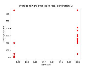
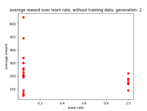
Additionally, it shows the that a low learning rate may allow for better performance as there are more dots to the left (lower learn rate) than there are to the right (high learn rate). Giving the AI’s learn rate parameter smaller values may allow it to train faster, especially with a smaller data set. Though this may not stop it from using the design flaw, I will keep it in mind when setting up the AI’s parameters to ensure that it can train faster.
Adding more varying values to the example generation
In this experiment to try and stop the AI from using the design flaw, I added more values to the learning rate and discount factor example generation, this was to see if there were any improvements in its exploration abilities while still maintaining a good score.

During the training, the AI seemed to work best with a learning rate of 0.05 as shown in the 2nd and 3rd generation graphs, these are shown below in fig 8 and 9.

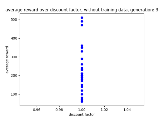
Additionally, the AI seems to have comes to a discount factor of 1 which is shown below in fig 10.
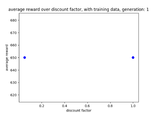
With the AI having a discount factor of 1 in its training data, it seems to explore the environment a lot more during the first game before using the flaw again in the second game. However, this seems to be at the expense of it achieving a high-score as this version only gains a score between 450 and 650 at best after 3 generations. This is compared to the previous version which got a score of 1200 after 3 generations but explored the environment less. A picture of the graph is shown below in fig 11 and its progress is shown in a video in fig 12.
Less discount parameters
Upon researching discount factors, one of the research papers suggested that having a smaller value would allow for better performance when exploring the environment (III and Singh 2020). When hearing about this I decided to give my discount factor examples smaller numbers (between 0 and 0.5) and a less amount of numbers in the example generation to see if this solution allows the AI to improve its performance after training. A picture of the AI’s smaller discount factor is shown below in fig 13.

Ideally if the AI could explore the environment more often and use the design flaw less often then the AI would be a success as it would play the game properly. Looking at how the AI plays the game, at this rate getting the AI to achieve a score of 1200 without using the flaw may be asking too much and instead achieving a score of 650 while playing the game properly would be a more achievable goal.
After training the AI for 3 generations the AI switches between 0.01 and 0.05 in order to achieve a score of 650. this is shown below in fig 14.

After using the training data on the AI, it would appear that having a smaller discount factor would cause it to use more efficient methods of playing the game, thus it used the flaw almost immediately. This can be seen in the video below in fig 15.
Graphs with different parameters and storage
As partly seen in the graphs above, I have now got the step total and discount factors plotted on scatter graphs and compared to the rewards. Alongside this I gave the graphs different colours: red for learning rate, blue for discount factor and green for step total, this improvement is to ensure the AI’s progress is more readable each generation.
While I was working on this, errors were coming up stating the sizes were different, however it turned out I simply forgot to clear the lists that where storing the data, causing new data to be added to the old data. With this solution the graphs worked perfectly though in order to make the solution more professional I might move the code to a function so that it looks neater.
Alongside this I stored the parameter data onto a csv file to ensure that the data could be viewed after training and plotted on a graph. A screenshot of the csv file is shown below in fig 16.

Further enquires
Looking at how the Genetic Algorithm (GA) optimization is used I wonder if it would be possible to add a database to the optimization and then use it to generate an average genome based on the performance of the individual. This could be a legacy system that keeps track of the best performing individuals 5 generations back and compares it to the current generation. This would be to see if anything from the previous generation could be used on the present to improve them, incase the AI starts dropping too much in performance. Of course this might cause problems with the mutation aspect of the GA, as it is meant to look for unique individual traits that could allow for better performance (GAD, 2018). However, I was curious if there was a way for unique traits to be applied to the next generation while ensuring the best traits of all the generations remain.
Reflection and conclusion
Reflecting on my work by experimenting with more values for the parameters allows for varying performance and scores. In addition, trying smaller values for the discount factor results in the AI being too efficient and picking a solution too quickly.
Looking at how the AI plays the game when not using overly efficient methods it may be difficult for the AI to get a score of 1200, so instead simply aiming for 650 could be a more achievable goal. Though it would be great if the AI could achieve big scores when playing the game properly, it feels inevitable that it would always use the design flaw to achieve its goal of high rewards.
Additionally, plotting more graphs to show how all the parameters are affecting the reward value and giving them different colours makes it much easier to follow the AI’s progress and tell which graph is which.
Looking at the AI’s performance it seems to either be doing well at the cost of overfitting and using illegal moves or playing the game more properly but at the cost of smaller scores.
Going further into my experimentation I would like to try giving the discount factor parameter, values that are between 0.5 and 1 to see if it will stop picking the most efficient method too soon. In addition, I might update the reward threshold to 1200 to ensure that the AI can train much faster, however this depends on the most frequent returned reward value.
Bibliography
III, Hal Daumé and Aarti SINGH. (eds.) 2020. Discount Factor as a Regularizer in Reinforcement Learning. PMLR.
GAD, Ahmed. 2018. ‘Introduction to Optimization with Genetic Algorithm’. Available at: https://towardsdatascience.com/introduction-to-optimization-with-genetic-algorithm-2f5001d9964b. [Accessed Feb 11,].
HILL, Ashley, et al. 2021. ‘Stable Baselines’. Available at: https://github.com/hill-a/stable-baselines. [Accessed 22/02/22].
Figure List
Figure 1: Max Oates. 2022. screenshot of reward threshold.
Figure 2: Max Oates. 2022. video of my AI exploiting a design flaw.
Figure 3: Max Oates. 2022. generation 1 of AI without training data.
Figure 4: Max Oates. 2022. generation 2 of AI without training data.
Figure 5: Max Oates. 2022. generation 3 of AI without training data.
Figure 6: Max Oates. 2022. graph of AI achieving a score of 1200.
Figure 7: Max Oates. 2022. picture of example generation.
Figure 8: Max Oates. 2022. generation 2 of training data.
Figure 9: Max Oates. 2022. generation 3 of training data.
Figure 10: Max Oates. 2022. discount factor after 3 generations.
Figure 11: Max Oates. 2022.example of discount factor graph using training data
Figure 12: Max Oates. 2022. example of AI getting a score of 450 while exploring.
Figure 13: Max Oates. 2022. picture of generation with a smaller discount factor.
Figure 14: Max Oates. 2022. graph of AI switch between different discount factors.
Figure 15: Max Oates. 2022. example of AI being efficient with a smaller discount rate.
Figure 16: Max Oates. 2022. example of parameter dat being used on the AI.
