In this post, I continue to train my AI while making improvements to the mutations aspect of the AI so that it will function better. During this I will make improvements to the graph to ensure the data is more readable.
Training improvements
After having a talk with my lecturer I realized instead of mutating the entire population I should just mutate a random part of one individual, thus giving more of a nudge rather than a push. Upon further inspection of my research that was definitely the case as the diagram in the previous post shows it just affecting one part of the individual’s genome and not the entirety. This is to ensure that offspring has its own unique traits while also retaining some traits of its parents to ensure the benefits of the parents’ genome is passed on to the offspring (Bryan 2021). A picture of the code can be seen below in fig 1.

This did partially stop the AI from overfitting, however it did still stay in a corner as it found that tactic was the most efficient strategy. This is due to it not losing any points from standing still for too long. Besides that the AI did occasionally move throughout the environment trying to gain a high score like a player would.
In its current state it can only seem to gain a score of 200 while moving through the environment but I have increased its mutation random number generator from -10 to 10 to -100 to 100. This was to see if it would allow for a great amount of performance and differentiation, but this did not prove to be the case and so the mutation random number was set back to -10 to 10 and was gaining a score between 200 and 650. In figs 3 and 4 the graphs below show this process, please note that during this point the title was pending on improvements.


I implemented a save and load feature that allowed the AI to save its training data and when the user felt the time was right, could enable the load feature so that the AI could train and improve itself further.
However there was a problem, for a time, the AI only seemed to score 200 points while still overfitting. This was because, I had noticed that the training data was causing the AI to give worse results than when it trained from scratch.
At first I tried to reposition the save and load code to see if the functions were being called before the training had started, thus affecting how the training data was being used and updated.
However, looking back at the plotted training data, I realized that the AI had a tendency to peak and then drop in performance at the end. This made me wonder if the reason the training data was giving off bad results was because it was saving the end bits of the data and thus overwriting previous and better training data. The progression and drop can be seen in fig 3. To solve this issue I tried to see if there was a way for it to ignore the drop and only save the training data during the progression stage.
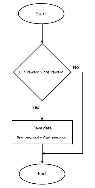
My solution was to have the AI compare its current reward to its previous reward and if the current reward was greater then its previous reward it would save the data. Below in fig 4 is a flowchart diagram of how the algorithm will work.
While it seemed simple at first, there was a problem, the variable containing the previous reward was being set back to 0 when the training function was being called. It did not matter whether it was global or local, the same results were happening. By having the previous reward variable set to global it would prevent Python from thinking the previous reward variable did not exist and needed to create a local variable in the function (Lutz 2014).
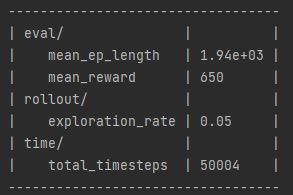
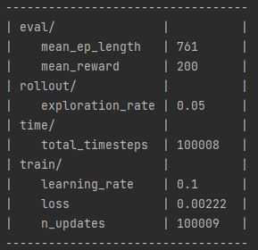
After some debugging it was clear that the global variable was working and it was being set to 0 by the current reward variable as that variable was switching between 0 and 50 during training and did not mimic the score in the game. This meant that I need to find a different way to get the agent’s reward. My temporary solution was to have the algorithm compare the number of steps the agent had preformed when training and see if the agent’s current steps were higher than the previous one. I used this method because usually if the number of steps are high, then so is the AI’s score, which is shown below in figs 5 and 6.
Additionally, getting the step total was much easier than getting the reward. After getting it set up, the save data algorithm could be more dynamic and work with other training sessions. This is shown below in fig 7.

I do want to try and see if I can get the algorithm to compare rewards as I’ve noticed cases where the AI can achieve a high reward with a small amount of steps. I could try evaluation_policy which is a function that can return reward values, however looking at its parameters, I’m unsure if it will create a separate environment or connect with the current one.
Nevertheless, saving the training data when it has a large number of steps seemed to have worked as by 3 generations and 5 iterations per generations, the AI was drifting between a score of 200 – 650. Continuing the training and loading the previous training data, by 6 generations the AI was constantly getting a score of 650 showing that it was progressing over time.
The last improvement I did for the training section was to add a discount factor to the AI’s parameters and GA optimization. This was to ensure that the AI would take risks and optimize its performance, as in its current form it was moving to one corner finding and concluding that this was the best solution too quickly. A discount factor is used in reinforcement learning to help reduce the number of steps required when training (François-Lavet et al. 2015). In addition, a discount factor can also be used to help optimize the performance of the AI, especially when using small amounts of data as it is the value that affects the AI planning horizon (III and Singh 2020). While this did show some improvement it did still overfit at times.
Graphs improvements
I began improvements on the graph so that it would only show the average step total and reward after every iteration. This was quite an easy process as I only needed to remove the code that called the plot function when an iteration was complete. Visualizing the progression data was much easier, as you now had only 3 to 4 graphs per iteration that showed the AI continuing in the new iteration from were it left off in the old one and either progressing or regressing. Additionally, I improved the title and labels so that their names were more descriptive of the data being shown.
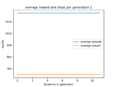
I then began to see if I could get the graph to show the average episode total and reward every generation so that the user only has to look at 3 graphs. Additionally, I adjusted the labels so that you could tell how many iterations had passed in the generation and which generation the graph was representing. Below in fig 8 is an example of the AI’s performance when using existing training data.
While talking about representation, to ensure that the data was readable, I set up a scatter graph to show the rewards that were being generated compared to their learn rate. In an early version the data was collected per iteration and while it did work, there was problem. For some reason, while the data was plotted, the title or labels did not appear, this is shown below in fig 9.

This is possibly due to something in the code affecting how the labels are displayed, instead of it being a size error on the x and y axis. The reason I believe this is the case, is because if the x and y axis did have different shapes then the graph wouldn’t have been built at all and an error would have appeared.
After looking at other examples of scatter graphs I found a solution by using MatplotLib’s subplots function. While subplots, as the name suggests, is meant for multiple graphs instead of one, it has proven to be a good solution and could be used properly in the future if I want to display multiple different datasets on one graph (Yim et al. 2018).
In fig 10 you can see a graph of the working scatter graphs and in fig 11 you can see the code used to make the graph.


As you can see in fig 10, the AI was making some progress with a learning rate of 0.01, however it got better results by using a learning rate of 0.5. This is visualised by the cluster of dots around a reward between 100 to 200 and a reward of 400.
Further enquires
All the systems have been set up properly to train, store and plot the AI’s data now and so I could begin working on seeing if the AI could be used in other Atari environments. In theory the AI would not need any changes due to the architecture of Stable Baseline3’s DQN AI as when setting it up to play Asterix (1983), it was able to run the environment and set up the states and actions with ease. My only concern would be how the graphs will plot the data as there could be a chance that the data would be stored differently, however this can only be found out with experimentations.
Reflection and conclusion
Upon reflecting on my work I am quite impressed with the AI performance as, though it may still be overfitting at times, its ability to get high scores almost constantly over time is very fortunate. However, as stated earlier, it does overfit at times, which I intend to try and fix or at least improve on by adjusting its discount factor parameter to ensure that it doesn’t pick an efficient path too soon. This would be done by first adding more examples to the example generator so that it has a larger array to choose from at the start of training.
As for graphs, having a scatter graph that shows how well the different learning rates are affecting the reward has been very helpful as it allows me to tell which learning rate works best. That being said, there are limitations, as at times it does show only two learning rates affecting the reward, however this may be due to the generations picking the best learning rate based on fitness. In addition, current graphs are the result of the AI using existing training.
If I have the time I would like to plot the step total and discount factor to the rewards as well to see how they affect the rewards as well.
In conclusion I will aim to improve the AI’s dismount timer to ensure that it is more explorative and does not overfit too soon. Alongside that I will aim to have the AI’s training from beginning to end put on a graph to see what the results will look like.
Bibliography
Asterix. 1983. Atari, inc, Atari, inc.
BRYAN, Graham. 2021. ‘Randomized Optimization in Machine Learning’. Available at: https://medium.com/geekculture/randomized-optimization-in-machine-learning-928b22cf87fe. [Accessed Feb 11,].
FRANÇOIS-LAVET, Vincent, Raphael FONTENEAU and Damien ERNST. 2015. ‘How to Discount Deep Reinforcement Learning: Towards New Dynamic Strategies’.
III, Hal Daumé and Aarti SINGH. (eds.) 2020. Discount Factor as a Regularizer in Reinforcement Learning. PMLR.
LUTZ, Mark. 2014. Python Pocket Reference . (5th edn). United States of America: O’REILLY.
YIM, Aldrin, Claire CHUNG and Allen YU. 2018. Matplotlib for Python Developers: Effective Techniques for Data Visualization with Python, 2nd Edition. Birmingham, UNITED KINGDOM: Packt Publishing, Limited.
Figure List
Figure 2: Max Oates. 2022. improved mutation code.
Figure 2: Max Oates. 2022. example of AI ranging from 650 to 200 points.
Figure 3: Max Oates. 2022. example of AI varying progressing.
Figure 4: Max Oates. 2022. Flowchart of save data algorithm.
Figure 5: Max Oates. 2022. example of greater step length with high reward.
Figure 6: Max Oates. 2022. example of smaller step length with small reward.
Figure 7: Max Oates. 2022. example of AI saving data when steps are higher.
Figure 8: Max Oates. 2022. example of graph of generation 1.
Figure 9: Max Oates. 2022. example of labels not appearing on scatter graph.
Figure 10: Max Oates. 2022. example of working scatter graph.
Figure 11: Max Oates. 2022. code used to plot scatter graph.
